
Linear Methods of Applied Mathematics
Evans M. Harrell II and James V. Herod
(Some remarks for the instructor).
version of 9 January 2000
If you wish to print a nicely formatted version of this chapter, you may download the rtf file, which will be interpreted and opened by Microsoft Word. Alternatively, you may switch to the Adobe Acrobat version of this chapter.
Some of the calculations of this chapter are available in a Maple worksheet or in a Mathematica notebook.
(Samples of the Maple worksheet and the Mathematica notebook are available here in a format which does not require either Maple or Mathematica.)
This course is concerned with some of the most important methods of applied mathematics, without which many technological developments of the nineteenth and twentieth centuries would have been impossible. When you have finished this course you will be able to solve most of the partial differential equations and integral equations that you are likely to encounter in engineering, and, just as importantly, you will understand what to expect from the solutions, which might emerge in a mysterious fashion from a computer at your workplace. You will also learn techniques that are useful in other contexts - Fourier series, special functions, and iteration.
The leitmotifs are the notions of linearity and orthogonality. By this stage in your education, you are familiar with vectors. You have added them by the head-to-tail construction, or by adding their components. You also know how to take their scalar (dot) product, producing a number equal to the product of the two lengths and the cosine of the angle between them:
One of the most powerful and astonishing ideas in modern mathematics is that in many regards functions can be treated just like vectors. (A bit of history.) There is a very close analogy between sets of functions and spaces of vectors, which will guide us to striking solutions for several of the most important differential equations you will use in science and engineering, especially the wave equation, the heat equation, and the potential equation.
Mathematicians have a way of making analogies without the mushiness that so often afflicts analogies in so many other contexts. It is called abstraction. While abstraction may sometimes seem like theory divorced from reality, when used properly it is a wonderful, and very practical, tool for solving problems.
This is why we will begin by making vectors abstract. Let us recall some facts about everyday vectors. If we have a bag full of vectors, we can scale them and add them together. We call the result a linear combination:
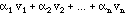
we'll normally use Greek letters for scalars (= ordinary real or complex numbers). It doesn't matter how many are in the combination, but unless we explicitly state otherwise, we will assume that it is only a finite sum, a finite linear combination. Of course, we can make linear combinations of functions, too:
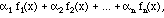
and the result is another function. In this way, the set of all functions is a vector space.
Definition I.1. More formally, a vector space over the complex numbers is a
set of entities, abstractly called vectors, for which
1. Any finite linear combination of vectors is a member of the same set
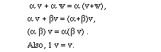
2. The usual commutative rule holds for addition: v + w = w + v,
3. Just for consistency, the usual commutative, associative, and distributive
laws hold for vector addition and multiplication by scalars. In other words
In practice the rules in 3 are obvious and not very interesting. From these
rules, you can show some other properties, such as:
There is a special element, which will be called the zero vector, equal to the
scalar 0 times any vector whatsoever. It has the property that for any vector
v, 0 + v = v.
For any vector v, there is a negative vector, called -v, such that v + (-v) = 0
(the zero vector).
Certain pretty reasonable conventions will be made, such as writing v - w
instead of v + (-
w).
Great - all the usual stuff works, right? Well, not quite. We don't assume
abstractly that we can multiply vectors by one another. Things like the dot
product and the cross product work for some vector spaces but not for others.
The other deep issue lurking in the shadows is infinite
linear combinations,
i.e., infinite series. Fourier liked them, and we'll see lots of them later.
But if the vectors are functions, perhaps the infinite series converges for
some x and not for others. For instance,
when x is a multiple of
1. The usual two-dimensional or three-dimensional vectors. It
makes little difference whether they are
thought of as column vectors such as
or as row vectors (2,3).
The set of all such
vectors will be denoted C2 or C3 (assuming complex entries are allowed -
otherwise R2 or respectively R3).
Mathematica
and Maple can perform all of the usual vector operations in a
straightforward way. (Review how this is done with
Mathematica or with
Maple.)
2. The set of complex numbers. Here there is no difference between a vector
and a scalar, and you can check all the properties pretty easily. We call this
a one-dimensional vector space.
3. The set Cn of n numbers in a list.
These are manipulated just
like 2- or 3- vectors, except
that the number of components is some other fixed number, n. For instance,
with C4, we might have elements such as (1,2,3,4) and (1,0,-1,-2),
which can be added and multiplied as follows:
(1,2,3,4) + (1,0,-1,-2) = (2, 2, 2, 2)
(1,2,3,4) . (1,0,-1,-2) = -10,
etc.
(Review how this is done with
Mathematica or with
Maple.)
4. The set of continuous functions of a variable x, 0 < x < 1. The
rather stupid function f0(x) = 0 for all x plays the role of the zero
element.
5. A smaller vector space of functions. Instead of simply listing n numbers,
let us multiply them by n different
functions, to define another vector space of functions. For example, for some
fixed n, consider
a1 sin(x) + a2 sin(2x) + ... + an sin(nx),
where the numbers ak can take on any value. Notice that this vector space is
a part of the one of example 4. In other words, it is a subspace .
6. The set of, say, 2 by 3 matrices. Addition means addition
component-wise:
7. The set of 3-component vectors (x,y,z) such that x - 2y + z = 0. This is a
plane through the origin.
Definitions I.3. A set of vectors {v1, ..., vn} is
linearly independent if it
is impossible to write any of the vectors in the set as a
linear combination of
the rest.
Linearly dependent is the opposite notion. The dimension of a
vector space V is the largest number n of linearly independent vectors {v1,
..., vn} which are contained in V. The span of a set {v1, ..., vn} is the
vector space V obtained by considering all possible linear combinations from
the set. We also say that {v1, ..., vn} spans V. A set {v1, ..., vn} is a
basis for a finite-dimensional vector space V if {v1, ..., vn} is linearly
independent and spans V.
Notice that the only way that two vectors can be linearly dependent is for them
to be proportional (parallel) or for one of them to be 0. If the set has the
same number of vectors as each vector has components, which frequently is the
case, then there is a calculation to test for linear dependence. Array the
vectors in a square matrix and calculate its determinant. If the determinant
is 0, they are dependent, and otherwise they are independent. For example,
consider the vectors {(1,2,3), (4,5,6),(7,8,9)}, which are not obviously
linearly dependent. A calculation shows that
Indeed, we can solve for one of these vectors as a linear combination of the
others:
Many of our vector spaces will be infinite-dimensional. For example,
{sin(nx)}
for n = 1, 2, ..., is an infinite, linearly independent set of continuous
functions - there is no way to write sin(400 x), for example, as a linear
combination of sine functions with lower frequencies, so you can see that each
time we introduce a sine function of a higher frequency into the list, it is
independent of the sines that were already there. An infinite linearly
independent set is a basis for V is every element of V is a limit of finite
linear combinations of the set - but we shall have to say more later about such
limits. A vector space has lots of different bases, but all bases contain the
same number of items.
For practical purposes, the dimension of a set is the number of degrees of
freedom, i.e., the number of parameters it takes to describe the set. For
example, Cn has dimension n, and the set of 2 by 3 matrices has six
elements, so its dimension is 6.
Model problem I.4. Show that the plane x + y + z = 0 is a two-dimensional
vector space.
The verification of the vector space properties will be left to the reader.
Here is how to show that the dimension is 2:
Solution. The solution can't be 3, since there are vectors in R3 which are
not in the plane, such as (1,1,1). On the other hand, here are two independent
vectors in the plane: (1,-1,0) and (1,1,-2).
(x,y,-x-y) =
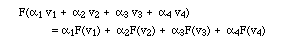
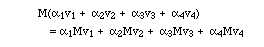
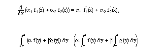
Definition I.5. A linear transformation is a function on vectors, with the property that it
doesn't matter whether linear combinations are made before or after the
transformation. Formally,
Linear transformations are also called
linear operators, or just operators for
short. You know plenty of examples:
Examples I.6.
1. Matrices. If M is a matrix and v, w etc. are column vectors, then
Think of rotation and reflection matrices here. If you put a bunch of vectors
head-to-tail and rotate the assemblage, or look at it in a mirror, you get the
same effect as if you first rotate or reflect the vectors, and then put them
head-to-tail. It may be less geometrically obvious when the matrix distorts
vectors in a trickier way, or there are more than three dimensions, but it is
still true. In this example, algebraic intuition might be more convincing than
geometric intuition
2. Derivatives and integrals. As we know,
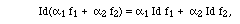
3. This may seem silly at first, but the identity operator Id, which just
leaves functions alone is a linear transformation:
since both sides are just round-about ways of writing
the effect of which on any vector is to leave it unchanged.
A linear transformation is a function defined on vectors, and the output is
always a vector, but the output need not be the same kind of vector as the
input. You should be familiar with this from matrices, since a 2 by 3
matrix acts on 3-vectors and produces 2-vectors. Similarly, the operator D
acts on a vector space of functions assumed to be differentiable and produces
functions which are not necessarily differentiable.
Example I.7. More exotic possibilities are possible, such as the operator
which acts on 2 by 2 matrices by the rule:
The whole theory we are going to develop begins with the analogy between
Example I.3.1 and Example I.3.2. We can think of the
linear operator of
differentiation by x as a kind of abstract matrix, denoted D .
If we also think of the functions f and g as entities unto
themselves, without focusing on the variable x, then the expression in the
first part of Example I.3.2 looks very much like Example I.3.1:
The custom with linear transformations, as with matrices, is to do without the
parentheses when the input variable is clear. It is tempting to manipulate
linear operators in many additional ways as if they were matrices, for instance
to multiply them together. This often works. For instance D2 = D D can be
thought of as the second derivative operator, and expressions such as D2 + D +
2 Id make sense. In passing, notice that if S is the integration operator of
the second part of Example 2, then D S f = f, so D is an inverse to S in the
sense that D S = Id. (But is S D = Id?)
Linear ODE's. In your course on ordinary differential equations, you studied
linear differential equations, a good example of which would be
D2y + Dy + 2y = 0
More specifically, this is an example of a "linear, homogeneous differential
equation of second order, with constant coefficients". We can picture this
equation as one for the null space of a differential operator A:
A y := (D2 + D + 2 Id) y = 0.
(1.1)
(Mathematical software can be used to conveniently define
differential operators;
see the
Maple worksheet or the
Mathematica notebook for this chapter.)
By definition, the null space N(A) is the set of all vectors solving this
equation; some texts refer to it as the kernel of A. There is no difference.
You may remember that the null space of a matrix is always a linear subspace,
and the same is true for the null space of any linear operator. E. g., the
plane of Example 1.2.6 is the null space of the matrix
What does this abstract statement about subspaces mean in a concrete way for
the problem of solving a linear homogeneous problem? It is the famous
superposition principle: If I can find two (or more) solutions of a linear
homogeneous equation, then any
linear combination of them is also a solution.
For matrices the general solution of the homogeneous equation is the set of
linear combinations of a finite number of particular solutions. This will also
be true for linear ordinary differential equations (the situation is a little
more complicated for linear partial differential equations). Indeed, the
number of independent functions in the null space of an ordinary differential
operator is equal to its order (the highest power of D). This is true even
when the coefficients are allowed to depend on x, so long as there are no
singularities (such as values of x where the coefficients become 0 or infinity).
Let us illustrate the situation with the two operators mentioned above.
Model Problem I.8. Find the null space of M as given in (1.2), which is the
same as finding the general solution of M v = 0.
In a linear algebra class you probably learned several techniques for finding
the solution vectors v, and the way you describe the null space may depend on the technique chosen.
Solution.
The nullspace can be found with software as a formula relating x, y, and z:
x = 2 y - z
Equivalently this is the
plane satisfying x - 2y + z = 0. This is a plane passing through the origin,
so it must be true that any linear combination of vectors in this plane again
lies in the plane. (Why is it important that the plane passes through the
origin?) A second way to describe the plane is to find a basis, i.e., two
independent vectors such as
v1 = (1,1,1) and
v2 = (1,0,-1),
which are both in the plane and which form a basis for it.
Model Problem I.9. Find the general solution of
A u(x) = 0.
(1.3)
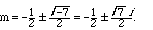
Solution. The method here is to guess a solution of the form emx, and
substitute to find what m must be. Usually, we find two possible values of
m, and in a class on ordinary differential equations we learned that the
general solution can be obtained from any two
linearly independent solutions (for
second order ODE's). If u(x) is of the form
emx, then A u = (m2 + m + 2) u, so
if u is not the zero function, we must have
Thus, two linearly independent solutions to (1.3) are
As these are complex valued - remembering
Euler's formula that
exp(i gamma) = cos(gamma) + i sin(gamma)
- they are not necessarily in the most convenient form. However, they can be
recombined easily into a pair of independent real functions,
The general solution is the span of these two functions, i.e.,
Finally, let us recall the solution of nonhomogeneous linear problems, and
observe how similarly it looks for matrix equations and differential
equations.
Model Problem I.10. Find the general solution of
Solution. The first step is to find a particular solution.
A bit of trial
and error leads to, perhaps,
There are many other, equally good choices for vp. The general solution is the set of
vectors of the form
so we see that the homogeneous solution is just added onto vp. The matrix M
annihilates the terms
The explicit answer is
Model Problem I.11. Find the general solution of
A u = exp(2x).
Solution. Again, the first step is to find a particular solution. Trial
and error with the guess
up(x) = C exp(2 x) leads to
A up = (4 + 2 + 2) C exp(2x),
showing us that we must choose C = 1/8, making
up = exp(2x) / 8.
The general solution is
u(x) = exp(2x) / 8 + a1 u1(x) + a2 u2(x).
where u1,2 are as given above.
(Mathematical software can of course solve Model Problem I.11 directly;
see the
Maple worksheet or the
Mathematica notebook for this chapter.)
Exercise I.1. For fluency with abstract vectors, use Definition I.1 to derive
the rules that followed the definition.
Exercise I.2. Verify that the spaces in Examples I.2 are all vector spaces.
Exercise I.3. Find which of the following are vector spaces and which are not.
In all cases, define addition and multiplication by scalars in the standard way.
a) The plane of vectors (x,y,z) such that x - 2y + z = 1.
b) The set consisting of the zero function and all functions for 0 < x <
1 which are not continuous at 1/2.
c) The set of 2 by 2 matrices with determinant 0.
d) The set of 2 by 2 matrices with trace 0. (Recall that the trace of a
matrix is the sum of all of its diagonal elements from upper left to lower
right.)
e) The set of 3 by 3 matrices with determinant 0.
f) The set of all polynomials in the variable x.
Exercise I.4. Show that a set {v1, ..., vn} is
linearly independent if and
only if the statement that
Exercise I.5. With the operators D and S as
defined in the text, acting
on the vector space consisting of all polynomials, is S D = Id? If not, give a
simple description of the operator SD.
Exercise I.6. (For review of ordinary differential equations.) Find the
general solutions of the following ordinary differential equations.
a) u'(t) = - 4 u(t)
b) u''(x) + (1/x) u'(x) - 9 u(x)/x2 = 0
c) u'''(x) = u(x)
Exercise I.7. Find the null space of the matrix
and find the general solution of
Exercise I.8. Find the null space of the differential operator
A = D2 - 2 D + Id
and find the general solution of
A u(x) = cos(x).

 ,
but it is certainly an improper sum when x =
/2,
and it is not immediately clear what happens for other values of x. What does
the series mean then? (We shall address this issue in
Chapter III.)
,
but it is certainly an improper sum when x =
/2,
and it is not immediately clear what happens for other values of x. What does
the series mean then? (We shall address this issue in
Chapter III.)![[2 3] transposed](pix/ch1x2.GIF)
![[1 0 i ] [2 -i 0 ] [3 -i i]
[-1 pi 2+i] + [-1 -pi 2-i] = [-2 0 4]
<p>
and multiplication by scalars affects all components:
<p>
[1 0 i ] [5 0 5i ]
5 [-1 pi 2+i] = [-5 5 pi 10+5i]](pix/ch1x3.GIF)
![In:= Det[{{1,2,3},{4,5,6},{7,8,9}}];
Out= 0](pix/ch1x8.GIF)
(7,8,9) = (-1) (1,2,3) + 2 (4,5,6)
Further observations. A general vector in the plane can be written with 2
parameters multiplying these two vectors, and it is not hard to find
the formula to express the general vector this way. First write the general
vector in the plane as (x,y,-x-y) (by substituting for z - notice 2 parameters
for 2 dimensions). It is a straightforward exercise
in linear algebra - with or without software - to solve for
 and
and
 such that
(1,-1,0) +
(1,1,-2).
We can solve this equation with the choices
= (x-y)/2 and
= (x+y)/2.
Hence the two vectors we found in the solution are a basis for the plane. Any
two independent vectors in the plane form a basis.
such that
(1,-1,0) +
(1,1,-2).
We can solve this equation with the choices
= (x-y)/2 and
= (x+y)/2.
Hence the two vectors we found in the solution are a basis for the plane. Any
two independent vectors in the plane form a basis.
 ,
1 f1 +
2
f2. The identity operator is a useful bit of notation for much the same
reason as the identity matrix,
,
1 f1 +
2
f2. The identity operator is a useful bit of notation for much the same
reason as the identity matrix, 
![F[{{m_11,m_12},{m_21,m_22}}] = m_11 sin(x) - 3 m_22 sin(2x)](pix/Ii.gif)

(See the
Maple worksheet or the
Mathematica notebook.)

 1 u1(x) +
2 u2(x).
1 u1(x) +
2 u2(x).
           [1]
     M v = [1]
           [1]

 j vj, so
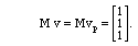
Compare with the following:
Exercises. , implies
that all the
's are zero.
, implies
that all the
's are zero.
             [1  4  7]
     M =     [2  5  8]
             [3  6  9]
             [1]
     M v =   [1]
             [1]
Link to
